mandizhao.github.io

A Fruitbot agent that Learns Fast and Generalizes Well

Introduction

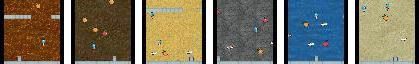
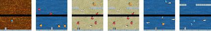
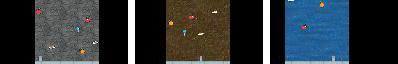
If a human player opens up Fruitbot (one of a series of Procgen games released by OpenAI) for the first time, they will see a moving game frame like one of these:

im1 im1

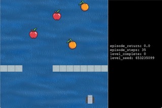
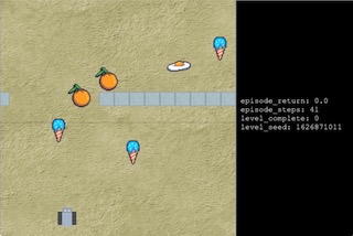
Without any description or clear-written rules, they can try moving the bot (shown on the bottom of the frame) left or right; and after a few trials and errors, they will quickly understand that, 1) hitting fruit objects increases the game score; 2) hitting a wall will kill the episode; 3) avoiding everything doesn’t change the score; 4) hitting non-fruit objects then the score goes down.

But now, instead of human players, we want to train the computer to play the game by itself – people in the field of aritificial intellengence are actively trying to solve this problem, because if you can teach the computer to play a simple game like this, you might be able to teach it more complicated games like Go or Dota, then, maybe you can teach robotic tasks such as grasping or moving objects, or even real-world missions like driving a car. The most popular and successful area of research in this field is reinforcement learning (RL); and thanks to recent advancements in deep neural networks, Deep Reinforcement Learning has been producing exciting results in all of the above mentioned tasks.

To put in more formal RL terms, this little bot we are trying to control is an agent, navigating in the game environment. The game frames we see is its observation, moving either left or right is an action, and positive game score is an reward. The colored frames indicate internal status of the game such as the bot’s location or its distance from an object, which we generally a state.

Now we can model the problem as a Markov Decision Process, the common underlying model for most RL problems. Note that 1) neither us human or the learning agent can see the internal state of the game, instead we see pictures, i.e. pixel inputs, i.e. observations, which often contain a subset of information about the internal state of the environment. 2) Fruitbot is a deterministic environment, which means the same states given the same actions will always produce the same reward and next states, no matter now many times we try. These settings make the game easy for us to play, however, it can have negative impacts on our training algorithm, therefore confuses the agent we trained with a slight twist in input.

Problem Setup

At a first glance, ProcGen environment resembles Atari games, the common pixel-based environment benckmarked by most deep RL algorithms; however, Procgen games pose additional challenges to test an agent’s ability to generalize. Fruitbot, one of the simplest games in Procgen, has a randomized observation domain by design.

Speficially, it has up to 100k different color-themes for the game frame, and different colors are called different “levels”. “Unseen levels” are new color themes, i.e. domains that will input the agent with pixel observations that its policy network hasn’t been trained on before. But all levels share the same game logic. The environment is designed to enable training (i.e. letting the agent interact with the enviornment) on only a subset of those levels, and testing a trained agent on unseen ones to see its performance.

Intuitively, if an agent plays anything like a human, it should be able to understand the color variation is irrelevant, and continutes to choose actions the same way as on seen levels.

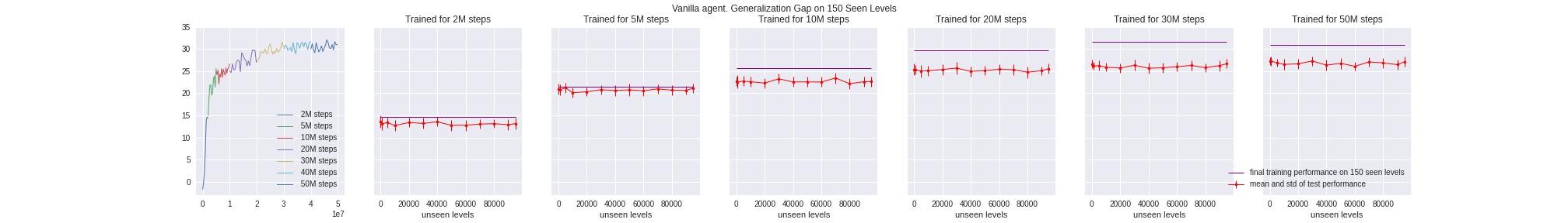
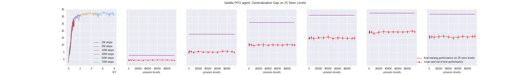
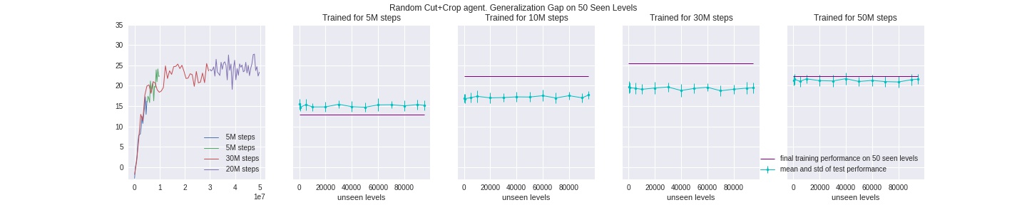
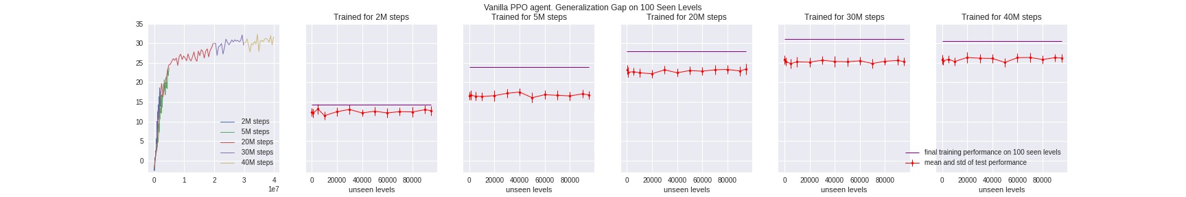
However, agents trained with the commonly-used, State-of-the-art deep RL algorithms will fail to recognize that. As a toy example and benchmark, we train a baseline PPO agent for up to 50 million timesteps (i.e. total steps taken in all parallel environments), and feed it with only 50 avaliable levels. As shown below on the left, the training performance on those seen levels consistently goes up and stablizes. However, then we test the trained agent at different sets of unseen levels, the agent performs consistently below its training score at the end of its training run.

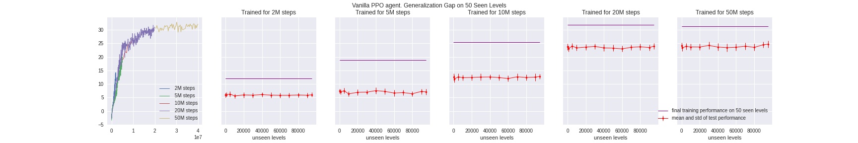
Note: Because the game has up up to 100k different levels, for all the testing runs above and below, for each run, we let a agent run for 1M timesteps across 1000 levels starting at level {100, 1000, 5000, 10000, …, 60000, 70000, 80000, 90000, 95000}, i.e. gather its scores on levels 100~1100, 1000~2000, 5000~6000, … 95000~96000, then take average and standard deviation of game scores for each set of 1000 levels tested.

This problem of overfitting has been identified and actively studied in recent deep RL research. It occurs because the baseline agent falsely correlates irrelevant observed informaion, i.e. the background color, with game reward. Training an agent that generalizes well to unseen domains is a challenging but necessary goal for any deep RL agent to succeed in the real world.

For this project, we call this performance difference between seen and unseen levels the Generalization Gap, and using a baseline PPO agent as benckmark, we present and analyze a set of data augmentation methods that are able to successfully close this gap.

Notes on the FruitBot Environment

To our best knowledge, the ProcGen game FruitBot, set to “easy” mode, has a (64,64,3) pixel-input of game frames, and the only source of randomness between different levels is the color-theme. So the notation “level” might be misleading: there isn’t new dynanmics or unseen food objects, and a “higher level” only means a different color background. Therefore we see very consistent test-time performance across different unseen “levels”.

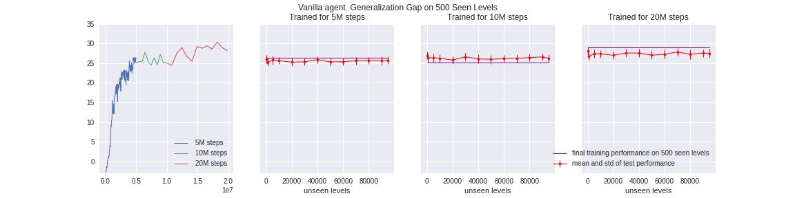
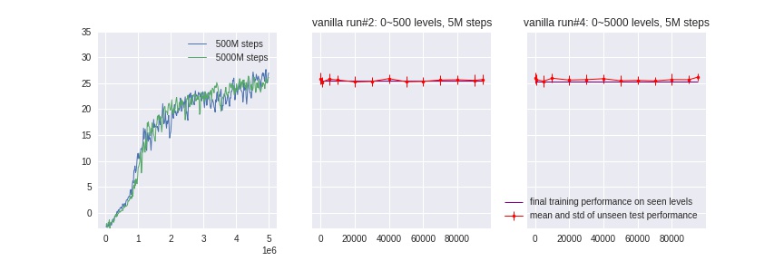
In addition, because the source of randomness comes purely from color-themes, even for a baseline PPO agent, only a relatively few number of seen levels is required (compared to 100k total avaliable levels) to learn well and close the generalization gap. We confirme this by training two PPO agent with 500 and 5000 seen levels, and test to show their performance on 5000+levels above. Therefore, we narrow down the generalization problem by “challenging” our agents to learn from only {25, 50, 100, 150} seen levels, and test on all other (100k - 150) levels.

Methods

At a high level, there are two general directions of methods we explored:

1) “Tough Love”: Confuse the agent first to make it generalize better later

These methods share the same idea but uses different tricks to add randomness to the agent input. Essentionally they are all randomizing the pixel inputs to block out some information in the observations, and in expectation, only the information that are least-affected by block-outs should be learned from. This way, the agent “forced” to learn generalizable representations instead of falsely correlating irrelevant elements to positive rewards (in Fruitbot’s case, color-themes)

2) “Handholding”: Encode pre-existing knowledge so that it learns relevant information faster,

Pre-process the pixel input so that the information we human know for sure is important (e.g. location of the bot) is “highlighted” for the agent to pay attention to. We will show some successful cases under this direction but choose not to explore further, because these methods require the same pre-processing during test time, therefore slowing down the experiment turnovers quite a lot.

Below we will show results and argue that, compared to a baseline PPO agent, roughly, approaches in 1) leads to a slower rate of improving during training time, but generalizes better at unseen levels. On the other hand, approach 2) improves the improvement rate during training (because some information is already encoded), but _not necessarily_leads to better performance at generlization.

Our code is avaliable at https://github.com/MandiZhao/train-procgen

1.a Random Edge Crop

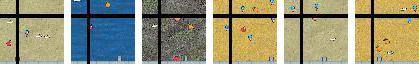
Randomly set two vertical strips, of total shape 15x64, on left and right edge of the image respectively, to zero pixel-values (i.e. black) before feeding the environment observations to agent’s policy network. In the example above, all images come from one batch of pixel inputs from six parallel environments, which get cropped at the same offset, but the crop is slightly different between each environment steps.

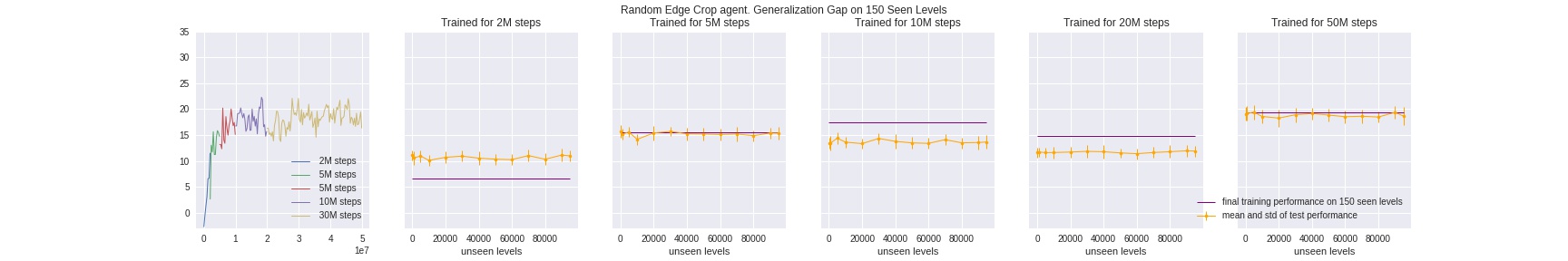
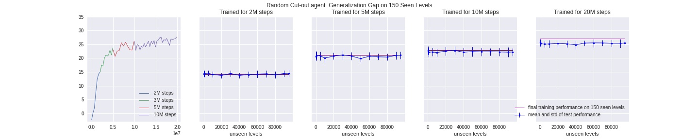
We train both an edge-crop and a vanilla agent on 150 levels, and compare their test-time results on unseen levels as explained above. As shown in the plots, although edge-crop led to slower improvement rate during training time, it’s better at closing the generalization gap, and is likely to further improve both in test and training performance if we train it for longer. Note that during test time we don’t do cropping at all, same for cut-out methods below.

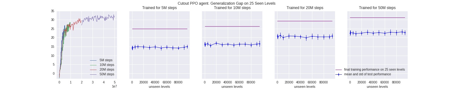
1.b Random Horizontal Cutout

Here we randomly cutout a fixed-sized horizontal strip, but added a little prior knowledge that the agent itself is always at the bottom of the frame: so we always cut-out a strip above the bottom ~10 pixels.

It’s important to note that, specific to this game, the location of agent/bot is fixed at the bottom of the frame, only allowed to shift left or right. Therefore we can’t do random crop like the RAD paper, crop a smaller square will just omit the bot completely. So instead I used a horizontal-only crop, i.e. randomly black-out 15 pixels on left and right edges of the frame, but not top or bottom. An example input:

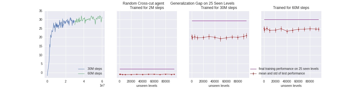
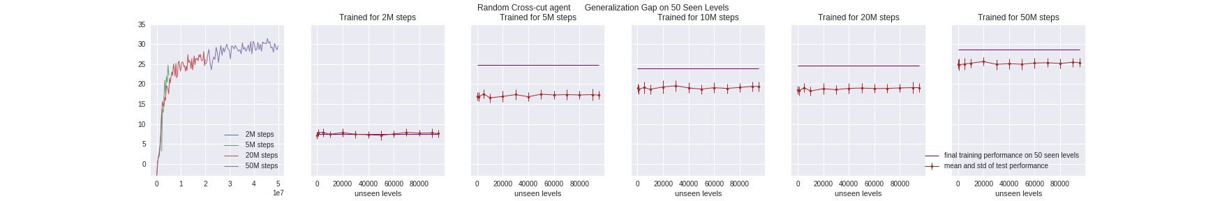
1.c Random Cross-like Cutout

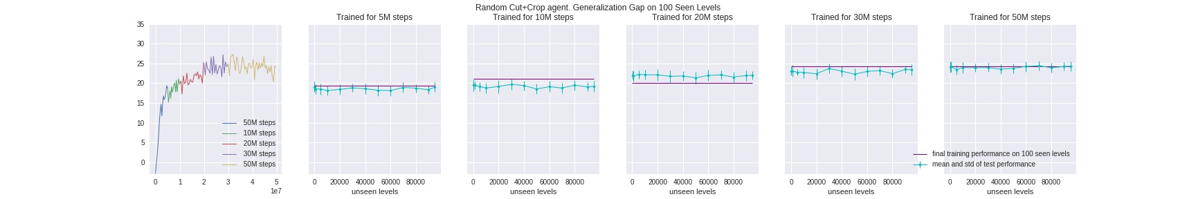
Similar to the two methods above, here for each batch of inputs, we randonly do a cross-cut: black out both a vertical and horizontal strip. Note that effectively we cut-out a bigger area than the above two, and by adding this “second degree” of covered areas, there are more different combinations in ways the cut-outs occur. This further prevents the agent to memorize all possible cut-out combinations, which is easier for the above two methods given sufficiently many training steps.

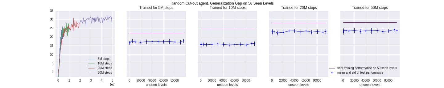
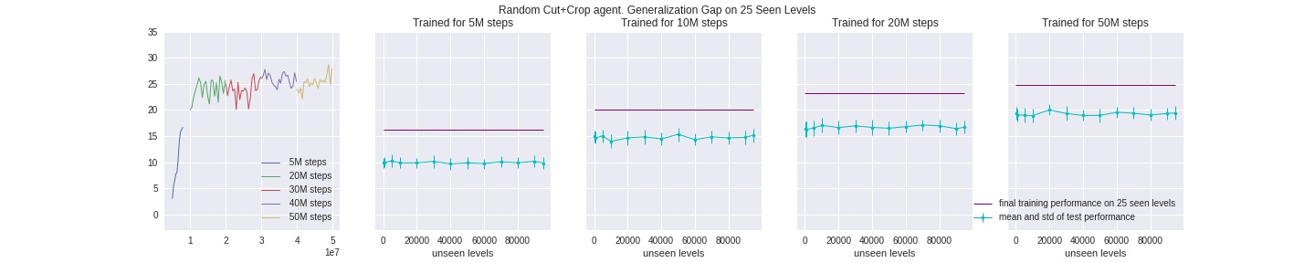
1.d Random Random Crop

As we can see, the above three methods still fell short at closing the generalization gap when trained on a scale of 50 million or more timesteps, which means the agent is still able to “memorize” and therefore overfit all the possible combinations of cut-out imaged. One way to account for this issue, similar to our reasoning above, is to add another layer of randomess by first randomly selecting one method from 1.a ~ 1.b above, generating its random offsets, and then applying the resulting cut-out to the batch of inputs. We omit an illustration here since it’s iterating over the above methods. We show that this method is best at closing the gap:

2.a Recenter

Inspired by this paper, we implement this method of re-centering for every pixel input: for each image in a batch (coming from different parallel enviornments), we scan the bottom pixels for a match of bot-colored object. Because the color-themes are different, pixel values of the bot object is also different for each level, although indifferentiable to the human eye. Thus we use a square-distance matching using one pre-saved bot patch’s pixel values, and locate the patch closest in value. After that, we re-center each image on a twice-sized dark background, so that the bot is always in the middle of the bottom rows.

Our locating-metric isn’t perfect, and some grey-ish color-themes make it extra difficult to identify the grey bot, as shown in the first image above. We did many sanity checks by saving the processed frames, and these error occur at a rather low frequency.

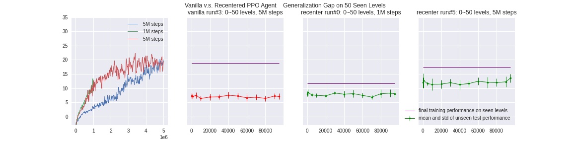
Recentering amounts to manually reinforcing the agent to focus on the bot’s location, which will be invariant given any color backgrounds. Because the agent learns faster the importance of bot patch’s location, we can see above that a re-centered agent takes way fewer timesteps to reach the same level of test/unseen performance than a vanilla PPO agent. However, if given few-enough levels, the re-centering will also run out of useful information, and the gap still occurs at longer training runs. Additionally, our implementation requires recenter-processing during testing time, which leads to a slower testing wall-clock time than other methods.

Conclusion

Put together, we compare all methods discussed above on the fewest-possible levels, all of them out-perform baseline PPO agents consistently:

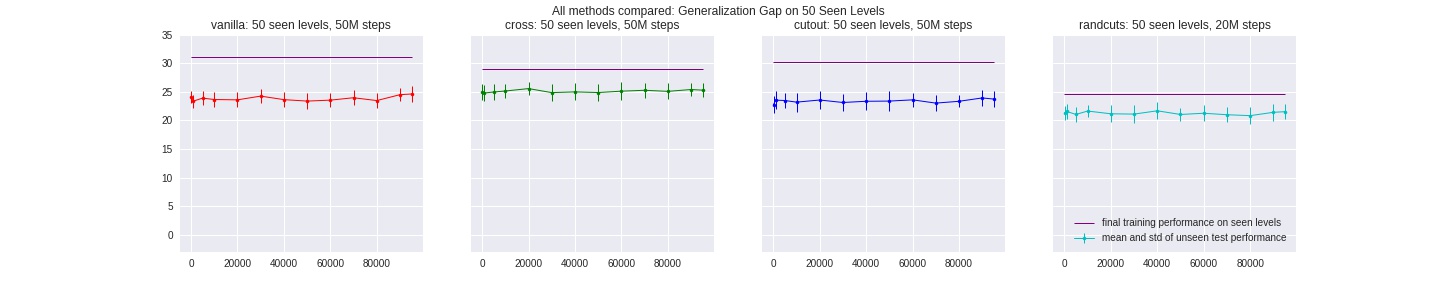
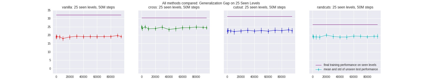
Our results confirm the idea that data augumentation methods tackles the problem of overfitting to randomized, pixel-based input domain. When training for sufficiently long, it is important to add and keep up the source of randomness in the way we augment/pre-processing the data, to prevent the agent from “memorizing” all possible inputs and overfitting to that augmentation method as well.

We were inspired by RAD, a comprehensive and state-of-the-art work on data augmentation, recently released and co-authored by our TA :). We recoginize that, as noted above, the randomness in easy-mode Fruitbot game doesn’t pose enough challenge in domain generalization, and some details of our method are specific to this game design, whereas RAD is tested on more complicated games. Our next-step would be using these augmentation methods in-bundle to reduce the amount of environment steps during training, as RAD proposed and succesfully implemented, therefore improving on data efficiency.

One major bottle-neck for this project is the limited computational resources, especially after expanding all experiments to 10 million scale. We’d like to thank the amazing Daniel Seita for his support in compute!

Rotation, Translation, and Cropping for Zero-Shot Generalization Change Ye, Ahmed Khalifa, Philip Bontrager, Julian Togelius arXiv:2001.09908

Reinforcement Learning with Augmented Data Michael Laskin, Kimin Lee, Adam Stooke, Lerrel Pinto, Pieter Abbeel, Aravind Srinivas
arXiv:2004.14990

Towards Interpretable Reinforcement Learning Using Attention Augmented Agents Alex Mott, Daniel Zoran, Mike Chrazanowski, Daan Wierstra, Danilo J. Rezende
arXiv:1906.02500

Network Randomization: A Simple Technique for Generalization in Deep Reinforcement Learning Kimin Lee, Kibok Lee, Jinwoo Shin, Honglak Lee arXiv:1910.05396

Proximal Policy Optimization Algorithms John Schulman, Filip WOlski, Prafulla Dhariwal, ALec Radford, Oleg Klimov
arXiv:1707.06347

Leveraging Procedural Generation to Benchmark Reinforcement Learning Karl Cobbe, Christopher Hesse, Jacob Hilton, John Schulman
arXiv:1912.01588

Observational Overfitting in Reinforcement Learning Xingyou Song, Yiding Jiang, Stephen Tu, Behnam Neyshabur
https://openreview.net/pdf?id=HJli2hNKDH

Appendix

Here we report experimental details, and other methods we explored but decided not to include in the main report.

Our code is based on the wonderful PPO implemntation from https://github.com/pokaxpoka/netrand https://github.com/openai/baselines

Benchmark Agent performance

As we can see, the agent’s generailzation ability improves as we increase the number of avaliable levels during training, we reason that this is due to the limited color-randomness unique to this game: if the agent sees enough (~500) different color themes, all the unseen levels/colors will have a bigger chance to resemble the colors that the agent has seen, e.g. an “unseen” light brown background can be similar to a dark brown background avaliable during training.

Random Random-cutout Agent (best performance)

Horizontal-cutout Agent

Cross-cut Agent

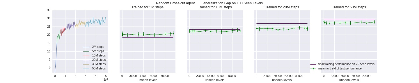
Learning from only the first 25 avaliable levels clearly (and intuitively) pose the most challenge for all agents, so we see the least improvement in this setting.

Note: For a better contrast and comparision, a more comprehensive list of experiments should be varying a fixed set of paramters along 2 dimensions for each agent, i.e. for each method, train an agent on {25, 50, 100, 150} seen levels for {2M, 5M, 10M, 20M, 50M, …} timesteps, then test it on {100, 1000, 2000, … 95000} intervals of unseen levels. This was what we set out to do; due to the very limited computational resources, we were able to only finish a subset of these trainings with sufficiently long testing evaluation, but we are confident these results make a valid conclusion.

All of our input-preprossing method are added on as plug-ins but keep the same underlying network architecture. For each training run, we followed a consistent set of hyperparameters:

num_envs = 64 
learning_rate = 5e-4
ent_coef = .01
gamma = .999
lam = .95
nsteps = 256
nminibatches = 8
ppo_epochs = 3
clip_range = .2
DROPOUT = 0.0
L2_WEIGHT = 1e-5

On top of the baseline PPO algorithm, we also added l2-norm that proves to be helpful in regularizing the network parameters, thus preventing it to overfit, and keeping our model size small (all of our models each take up 2.5MB whereas a baseline PPO model takes up 7.5MB)